A Neural Net Model for Distillation with Weights Explained

Large models in deep learning show unprecedented capabilities in generating human-like language, realistic images, and even videos. Developing an understanding of what information is distilled in their weights is important for their safe deployment.

In our NeurIPS 2023 paper, we studied a natural non-linear deep learning model – shallow neural net – in a distillation setting. This neural net model is simple enough that every single neuron of the trained network is interpretable. Yet it is non-linear and has a finite size, making its mathematical analysis very challenging. As the width increases, the learned weights show an intriguing phase transition: the solution implemented by the neural net fundamentally changes structure.

In this blog post, I will give an intuitive exposition of our paper and present some of the fascinating open questions on interpretability and phase transitions of neural nets. If you like toy models of superposition or pizza and clock, you might enjoy reading this blog post!

Motivation

Large models of 2024 are trained by using massive amounts of structured data. Arguably, even though these models have billions to trillions of parameters, they nevertheless fall short of learning the true distribution of data which is typically the whole Internet. This begs for a systematic study of neural nets with limited capacity.

Moreover, interpretation of what knowledge is encoded in trained models and how is important for the safe deployment of large models.

We propose to study a toy model of neural networks where each learned neuron has a simple interpretation. Similar neural structures are also found in toy models of superposition.

Setting & Phenomenology of the Model

We aim to study a non-linear neural network with a limited capacity that remains simple enough to allow for a thorough mathematical analysis. To ensure that the neural net has a limited capacity, we install another neural network with a larger width to generate targets from inputs. The first neural net is also called the student as it learns from the targets generated by the teacher. The goal of the student net is to compress the weights of the teacher net optimally.

Specifically, the student neural network is a two-layer feedforward module
\begin{align} f(x) = \sum_{i=1}^n a_i \sigma (w_i^T x) \end{align} where $ \sigma $ is a non-linear activation. We aim to express and interpret every neuron $(a_i, w_i)$ in a trained network. We use erf

\begin{align} \sigma_{\text{erf}}(x) = \frac{2}{\sqrt{\pi}} \int^{\frac{x}{\sqrt{2}}}_0 e^{-{t^2}/2} dt \end{align}

and ReLU activations $\sigma_{\text{ReLU}}(x) = \text{max}(0, x)$.

Naturally, weights in a trained net will encode the structure of the target function and input data distribution and how exactly this happens depends on the activation function. See Assumptions for the teacher model, input distribution, and activation function we considered and for a discussion of the generality and limitations of these assumptions.

We experimented with teacher networks of width $k = 3,…,100$ and student networks of width $n \leq k$. All neural nets are trained with gradient flow using MLPGradientFlow.jl which is a customized package for the teacher-student problem. Let’s visualize the weights for a trained student net.

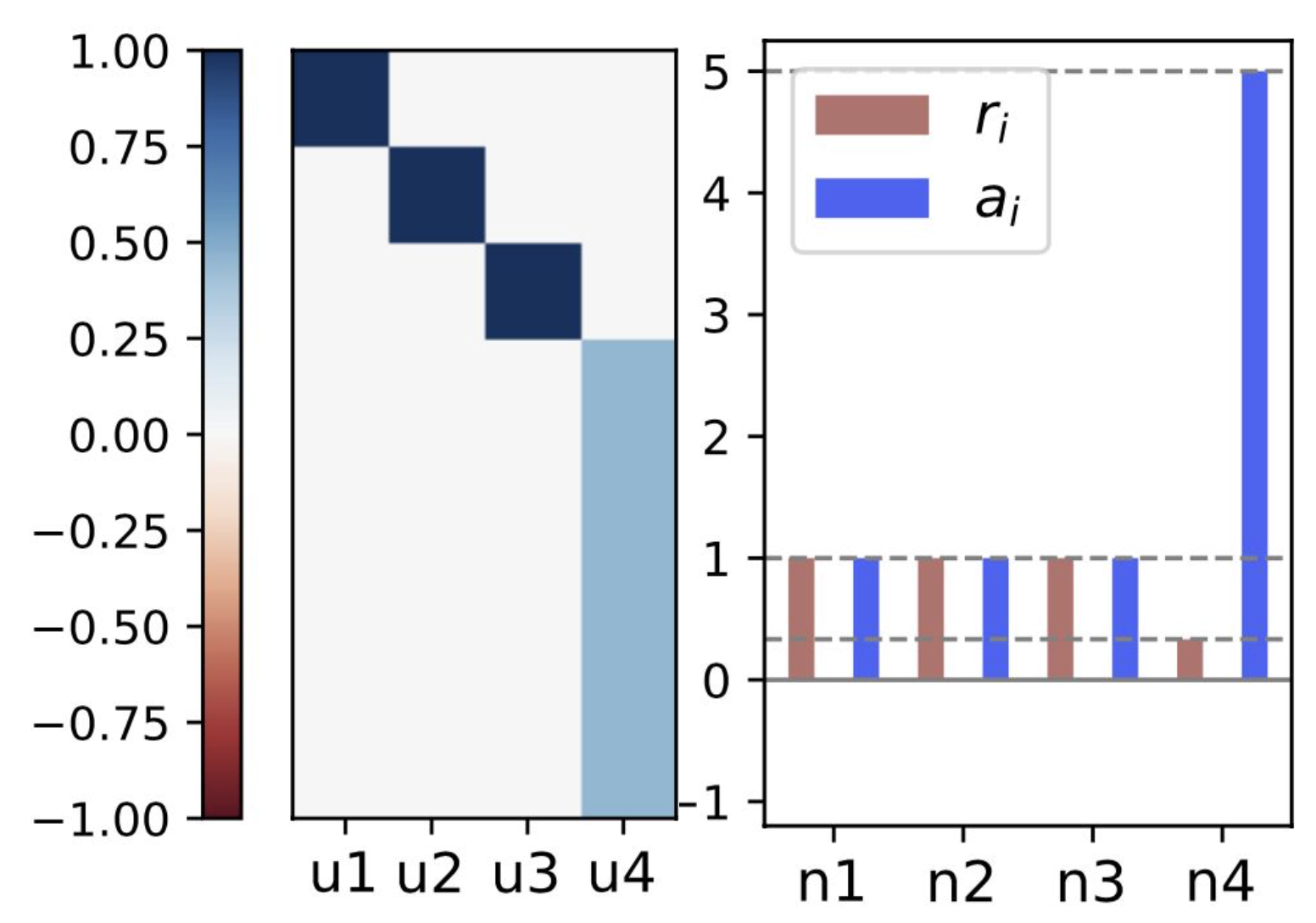
In all experiments, all trained nets can be explained with four types of neurons

• Exact copy neuron
• Exact average neuron
• Approximate copy neuron
• Approximate average neuron

We found exact copy and average neurons when using erf activation and when the width satisfies $n<\gamma_1 k $ for a certain fraction $\gamma_1 \sim 0.46$. Changing the activation to ReLU or using a bigger width resulted in similar neurons that we interpret as perturbations of the exact copy and average neurons. In this blog post, we focus on explaining the exact copy and average neurons phenomenologically and mathematically, and we call them simply ‘copy’ and ‘average’.

• When the width is smaller than a certain fraction of the target width ($n< \gamma_1 k$), for all random initializations, the neural net converges to a special configuration: $n-1$ neurons copy $n-1$ of target neurons and the $n$-th neuron implements an average of the remaining ones (see Fig 1). One might wonder why the network does not prefer other partitions of $k$ target neurons into $n$ by using more average neurons.

• See Results for the exact construction of all such ‘copy-average’ configurations and to see that these are critical points of the loss landscape. Moreover, we proved that the optimal copy-average configuration uses exactly one average neuron. Hence a configuration with $(n-1)$ copy neurons and one average neuron is called C-A optimal.

• Surprisingly, when the width is larger than another fraction of the target width ($n>\gamma_2 k$), for all random initializations, the neural net converges to another special configuration where each of its neurons implements an approximate copy of $n$ of target neurons. We called this configuration perturbed-$n$-copy and denoted it by P-$n$-C in short.

• When the width is in between these two fractions, we observe that the network converges to either a C-A optimal or a perturbed-$n$-copy configuration, depending on the direction of the initialization.

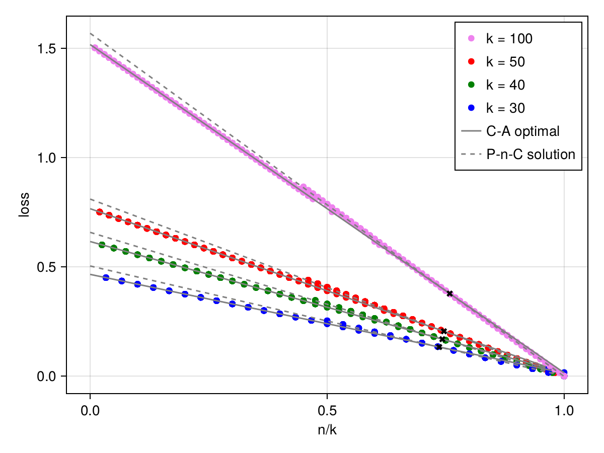
We are excited to observe a phase transition in learned weights as its width gets larger. A phase transition of the solution of a neural net as width grows is observed also for algorithmic tasks (see eg. pizza and clock).

Moreover, we observe that the change points correspond to certain fractions between student and teacher widths $n/k$, i.e. as $k$ approaches infinity, the width for which the student network converges to a different solution, at least for some random initializations, approaches to $\gamma_1 k$. However, computing gradients for every pair of neurons is costly and we could run this experiment only up to target width $k=100$.

Assumptions

We will use a commonly studied teacher model since the Saad and Solla paper from 1995 \begin{align} f^*(x) = \sum_{j=1}^k \sigma (v_j^T x) \end{align} where $ v_j $'s are orthonormal (unit norm and orthogonal). The target is equally influenced by each of the teacher’s vectors in this model. The input distribution is assumed to be standard Gaussian $ x \sim \mathcal{N}(0, I_d) $.

This model is doubly symmetric due to the symmetry of the input distribution and the true function hence it is not suitable to study feature importance or data anisotropies. However, this model is very appealing to studying non-linear neural nets of finite width and might serve as a first step before moving on to more complicated models. We discuss the generality and limitations of these assumptions below.

• In large input dimensions, one can expect that Gaussian universality to kick in: the learned weights do not depend on the higher moments of the input distribution. On the downside, structured data is not expected to have isotropic covariance, but probably a thorough analysis of the isotropic covariance is the first step.

• Any true function can be approximated arbitrarily well with a large enough neural net thanks to the universal approximation theorem. Hence assuming that the true function itself is a neural net is not too bad (basically dropping some tail properties of the targets). Assuming the teacher net has no bias and equivalent neurons in orthogonal directions however might be too simplistic and it’d be great to relax this in the future.

Importantly, we rely on the nice analytic properties of the erf activation for the mathematical analysis in the next part. We refer to our paper for experiments with ReLU activation. Interestingly, the network employs a very similar strategy of learning an optimal C-A point or a P-$n$-C point for the same width brackets. The difference is that the ReLU-net implements approximate copy and average neurons, making its mathematical analysis more difficult. See these papers for attempts to crack the ReLU nets.

Results

I will informally present the results of the multi-neuron nets from our paper.

Construction of Copy-Average Neurons

First, let us write out the definitions of copy and average neurons.

• Copy neuron is a student neuron that exactly replicates the weights of one of the target neurons, that is \begin{align} (w_i, a_i) = (v_j, 1) \end{align}

• Average neuron is a student neuron which is the global optimal in approximating the sum of target neurons, that is \begin{align} (w_i, a_i) = \text{argmin} \ \mathbb{E}_{x \sim \mathcal{N}(0, I)} [(a_i \sigma (w_i^T x) - \sum \sigma(v_j^T x))^2]. \end{align} In particular, for a family of activation functions for which the linear component is dominant in the Hermite basis, which includes erf, ReLU, softplus, tanh, the global minimum of the above problem satisfies

\begin{align} a_i \geq k, | w_i | \leq \frac{1}{\sqrt{k}}, \frac{ w_i }{ | w_i |} = \frac{1}{\sqrt{k}} \sum_{j=1}^k v_j. \end{align}

Copy-Average Configurations are Critical Points

Let us choose an arbitrary partioning of $k$ teacher neurons into $n$ non-empty buckets denoted by $(\ell_1, …, \ell_n)$. The network weights for this partition are

\begin{align} (w_i, a_i) = \text{optimal approximation of} \sum_{j \in [S_i]} \sigma(v_j^T x) \end{align}

where $S_i$ constains indices between $(\ell_1+…+\ell_{i-1}, \ell_1+…+\ell_i)$. We call all such configurations copy-average as they are a combination of copy and average neurons.

We proved that all copy-average configurations are critical points of the multi-neuron loss landscape. This is quite relevant since

• As training trajectories are attracted by saddle points, these fully interpretable configurations likely guide training and might be the final network weights in case of early stopping

• Training parts of the neural net using the partitions of the targets is a much more efficient training scheme and magically does not cost any loss of performance

Optimal Copy-Average Configuration

We have a new family of critical points each representing compression schemes corresponding to a different partition. We wonder which one is optimal.

The first-layer vectors $w_i$ of copy-average configurations are orthogonal to each other. This is not trivial, in fact, we introduced an equivalent constrained optimization problem to prove that $w_i$ is in the span of the target vectors in the corresponding index set. Moreover, thanks to the rotational symmetry of the Gaussian measure, the loss of a copy-average configuration is

\begin{align} L(\ell_1, …, \ell_n) = L(\ell_1) + … + L(\ell_n) \end{align}

where $L(\ell_i)$ is the optimal loss, or the approximation error, of the one-neuron network when learning from a teacher with $\ell_i$ neurons. Finding the optimal partition minimizing the above objective is a combinatorial optimization problem that is in general very costly, or impossible to solve.

However, for erf activation, we proved that $L(\ell_1)$ is a discrete concave function, which implies

\begin{align} L(1) + L(\ell_1-1) \leq L(\ell_2) + L(\ell_1 - \ell_2). \end{align}

In words, if there are two buckets both with more than one neuron in the student network, redistributing the neurons so that there is exactly one neuron in one of the buckets decreases the loss! We conclude that in the optimal C-A configuration, there is exactly one average neuron and the others are copy neurons.

Open Questions

In this work, we think we might have pinpointed a non-linear neural net model that shows complex phenomena and at the same time allows for a mathematical analysis. This opens up many exciting questions and research avenues

In our setting

• Can one prove convergence to an optimal C-A point for widths not exceeding a certain fraction of the teacher width?

• Can one prove converge to a perturbed-n-copy point for widths exceeding a certain fraction of the teacher width?

• For the widths in between the two fractions of the teacher width, can one show that both optimal C-A points and perturbed-n-copy points are local minima?

• Can one prove that the global optimum is an optimal C-A point for widths not exceeding a certain fraction of the teacher width? Or, can one dispute this conjecture by showing that are there other minima that achieve a lower loss?

• Can one give a general characterization of copy-average configurations for general activation functions?

Generalizations

• Does the trained neural network learn to copy and average neurons when

  • the input distribution is anisotropic,
  • the teacher vectors are not equivalent, for ex. different norms.

• Is there a fundamental link between monosemantic and polysemantic neurons in toy models of superposition and copy and average neurons discussed here?

• Can neural networks be trained using combinatorial optimization? For ex. by partitioning the targets into pieces, training sub-networks separately to learn the pieces, combining the sub-networks, and possibly fine-tuning.

Acknowledgements

I thank the co-authors of the paper, Amire, and Wulfram, for many discussions that helped digest the results. Hopefully, this exposition is now intuitive thanks to them and many others, I was fortunate to discuss with after I moved to NYU and Flatiron CCM. Special thanks to Johanni for making Figure 2 for this blog post and for his constant energy and support during the making of the results.